CUDA MMA (Matrix Multiply Accumulate) and the Roofline model

Graphical Processing Units (GPUs) are hardware accelerators for compute, when writing an algorithm we want to squeeze the most of our machine, i.e. we want to maximize the number of floating point operations per second (FLOPs/s). In this post we will learn about the Roofline Model, a model that helps us understand how general compute works and we will learn a few tricks to maximize FLOps in a GPU. This will be done with real kernel examples for matrix multiplication and addition (MMA) whilst computing the roofline curves for each kernel in an A100 GPU (used Thunder Compute cloud provider).

This post is inspired by the Siboehm post about GPU matrix multiplication.

All the code can be found in the blogging code and specifically in the section cuda-mma.

Definitions in computation

• Floating Point Operations (FLOPs) is the total count of floating-point arithmetic operations i.e. additions, multiplications, fused multiply-accumulate (FMAs) opearations that need to be done to complete a task. For instance, a matrix multiplication of two matrices with sizes $M \times K$ and $K \times N$ we need to do $M \times N \times (K-1)$ operations (explained in CUDA Matrix Multiplication).
• Throughput The rate at which a processor can execute operations, typically measured in FLOPs/second (FLOP/s), commonly expressed as GFLOP/s or TFLOP/s. This is what you’re actually measuring when you benchmark a kernel’s compute performance
  • Peak theoretical throughput: the hardware’s maximum possible rate (from spec sheets), e.g. an A100’s peak FP32 or TF32 throughput.
  • Achieved throughput: what your kernel actually hits in practice.
• Arithmetic/Computational Intensity: The ratio of compute work to memory traffic, or in more simple terms, how many floating point operations do we need to do per byte of information accessed from memory. It’s measured in FLOPs per byte (FLOPs/byte). For instance, the number of bytes moved for the matrix multiplication would be $s$($M \times K$ + $K \times N$ + $M \times N$) where inside the parentheesis we have the sizes of the matrices and $s$ is the size of the elements (4 for float, 8 for double). The ratio of the total floating point operations to the total size is the arithmetic intensity.
• Memory Latency: The time between issuing a memory request and the requested data actually becoming usable at the compute level. The farther away from the compute unit the more latency (e.g. registers have low latency).
• Memory Bandwidth: The rate at which data can move between memory (HBM/DRAM) and the compute units, measured in bytes/second (GB/s or TB/s). Bandwidth is higher closer to the compute units.

The tradeoff memory bound vs compute bound

Every processor has the same basic problem: it can only do math as fast as it can get data. A GPU core can do a multiply-add every clock cycle, but only if the two numbers it needs are already sitting in a register. If they have to be fetched from memory, the core stalls and waits. This is true for laptop CPUs, server CPUs, and GPUs alike — what differs across hardware is just how fast the memory and compute are, not the tension between them.

Picture a worker stationed on an assembly line (a CPU in the analogy). Parts arrive on a conveyor belt (memory BUS) from the warehouse, the worker does some operation on each part, say drilling $N$ holes in each piece, a process that takes takes $kN$ seconds. This is the arithmetic intensity, the amount of work per piece (or byte) the worker does. The arithmetic intensity is low if the worker has to drill less holes per piece or large if he has to drill more holes. Le’ts assume the conveyor belt can deliver items at a fixed rate of $P$ items per minute.

The system will be memory bound if the belt brings parts slower than the worker can process them; In this scenario the worker will be sit idle every time he finishes a piece waiting for the next one. We are underperforming. The limiting performance factor is the conveyor belt speed (or the memory transfer speed).

In another case the system can be compute bound, this is, when the work intensity is very high (the worker has to drill many holes per piece, i.e. we do more computation per byte) but the conveyor belt is fast. In this case the worker cannot drill faster, we reached the maximum drills per minute (floating point operations per minute) that the sytem can deliver. The items just wait there to be processed as close as it’s possilbe to the worker (deeper levels of memory ideally).

Introducing the Roofline Model where we will see the two regimes. In the $x$ axis we represent the aritmethic intensity and in the $y$ axis the performance. Smaller intensity means less floating point operations per byte transferred, e.g. a simple addition of two numbers has very low computational intensity whereas adding two numbers $N$ times is higher intensity (yes, silly operation but just for you to get the idea). In the regime of small intensity we are memory bound, the processor can do the work faster than the byte is delivered so it yields a small performance (smaller FLOPs/s). For large arithmetic intensity we keep the processors busy at all times and therefore the number of floating point operations increases reaching to a plateau that corresponds to the maximum “theoretical” performance of the processor. In the schematic graph above we can see the areas where we are memory bound and which are compute bound. The ridge point is defined as the transition point where the compute goes from memory bound to compute bound and vice versa.

As an example, here are the numbers for an Nvidia A100 GPU (spect sheet) for different floating point operations and type of cores.

Math mode	Peak throughput
FP32 (regular cores)	19.5 TFLOP/s
TF32 (Tensor Cores)	156 TFLOP/s
FP16 (Tensor Cores)	312 TFLOP/s
FP64 (Tensor Cores)	19.5 TFLOP/s

What we explained in this section is obviously and oversimplification, a generalization that applies to all types of compute (CPU, GPUs…) but without taking into detail specific architectures. As a general guide, always bring the data as close to the compute node as possible and maximize computational intensity if possible to reach peak peformance. In GPUs specifically we can hide memory latency by fusing kernels (less calls/waits for CPU) and memory coalescing (threads in the same warp load consecutive data).

Roofline curves for SGEMA on a A100

In this section we are going to calculate the experimental roofline model for several kernels for single precision general matrix multiplication and accumulate (SGEMA) operation.

SGEMM’s arithmetic intensity

SGEMM (Single-precision General Matrix Multiply) computes $C \leftarrow A \cdot B + C$ for matrices of 32-bit floats (4 bytes). For square matrices of size $S \times S$:

• Operations: $2S^3$ (one multiply and one add per entry of the inner product sum).
• Memory traffic: $4 \times S^2 \times 4 = 16S^2$ bytes — one read each of $A$, $B$, $C$, and one write of $C$, each of $S^2$ floats at 4 bytes each.
• Arithmetic intensity: $I(S) = 2S^3 / (16S^2) = S/8$ FLOPs/byte.

Therefore the arithmetic intensity increases linearly with the matrix size. There is a reason why I chose matrix multiplication, try to do the same calculation with vector addition (solution: the compute intensity does not depend on the vector size, but do the numbers yourself!).

For our matrix multiplication example $S/8$ FLOPs/byte is the best-case intensity — assuming perfect data reuse so each matrix element is read exactly once. A naive implementation that re-reads $A$ and $B$ from main memory on every step of the inner loop falls far below this. Tiling (loading chunks into fast shared memory), thread coarsening (having each thread compute more output values), and Tensor Core MMA instructions are all techniques for pushing the actual intensity back toward the theoretical $S/8$.

CUDA custom kernels for SGEMM

In this subsection we will explain the different kernels implemented for the SGEMM operation. Our CPU equivalent is the function cblas_sgemm whose signature is

func cblas_sgemm(
    _ ORDER: CBLAS_ORDER,
    _ TRANSA: CBLAS_TRANSPOSE,
    _ TRANSB: CBLAS_TRANSPOSE,
    _ M: __LAPACK_int,
    _ N: __LAPACK_int,
    _ K: __LAPACK_int,
    _ ALPHA: Float,
    _ A: UnsafePointer<Float>?,
    _ LDA: __LAPACK_int,
    _ B: UnsafePointer<Float>?,
    _ LDB: __LAPACK_int,
    _ BETA: Float,
    _ C: UnsafeMutablePointer<Float>?,
    _ LDC: __LAPACK_int
)

and calculates

\[C \leftarrow \alpha AB + \beta C\]

with optional use of transforms of $A$, $B$ or both. We will ommit the order (assuming all matrices are row-order), transpose parameters and leading dimensions.

We are benchmarking the validity of the results of our kernels using this cblas_sgemm function for square matrix multiplication. In this section we will explain several kernels and calculate it’s roofline curves.

Naive SGEMM

Let’s jump straight to the kernel code for the most simple calculation, the naive kernel

__global__ void sgemm_naive(
    size_t M,
    size_t N,
    size_t K,
    float alpha,
    const float *A,              // [M x K] row-major
    const float *B,              // [K x N] row-major
    float beta, 
    float *C)                    // [M x N] row-major  (in-out: C = alpha*A*B + beta*C)
    {                   
    
    const uint x = blockIdx.x * blockDim.x + threadIdx.x;  // 0 .. M-1 (Rows of C)
    const uint y = blockIdx.y * blockDim.y + threadIdx.y;  // 0 .. N-1 (Columns of C)

    // Warp access e.g. warp 0:
    // x is consecutive for threads 0..31, y is the same for threads 0..31
    // each warp accesses a column of C, with non-coalesced accesses to A and C, but broadcast access to B
    // Ref: https://siboehm.com/articles/22/CUDA-MMM

    if (x >= M || y >= N) return;

    float acc = 0.0f;
    for (size_t i = 0; i < K; ++i){
        acc += A[x * K + i] * B[i * N + y];
    }

    C[x * N + y] = alpha * acc + beta * C[x * N + y];
}

This kernel is called from device as

dim3 gridDim(CEIL_DIV(S, 32), CEIL_DIV(S, 32));
dim3 blockDim(32, 32, 1);
sgemm_naive<<<gridDim, blockDim>>>(S, S, S, 1.0f, d_A, d_B, 0.0f, d_C);

for simple matrix multiplication where S is the size of the square matrices A, B and C. See that the rows (x) and columns (y) are defined per thread:

const uint x = blockIdx.x * blockDim.x + threadIdx.x;  // 0 .. M-1 (Rows of C)
const uint y = blockIdx.y * blockDim.y + threadIdx.y;  // 0 .. N-1 (Columns of C)

Each thread will calculate an element of the matrix C. Won’t get into the details of high level CUDA programming and blocks and threads, I have explained that in a previous post, also there is plenty of documentation.

As you can imagine, this kernel is extremely inefficient. The first inefficiency is memory access: for the GPU to access memory efficiently, consecutive threads should access consecutive addresses. When this happens, the GPU can service the entire warp with a single wide memory transaction instead of many small ones, which reduces total transfer time. Let’s examine warp 0 for a block:

x = blockIdx.x*32 + (0..31) → varies 0..31
y = blockIdx.y*32 + 0 → fixed

Consecutive warp threads are filling in rows of C first. Let’s examine the memory accesses for consecutive threads:

• A: A[x*K + i]: x varies, i fixed for the iteration → addresses are 0K+i, 1K+i, 2*K+i, … — spaced K floats apart. Strided / not coalesced. Up to 32 separate cache-line fetches.

• B: B[i*N + y]: i fixed, y fixed → every thread in the warp computes the exact same address. That is called a broadcast. One transaction serves all 32 threads — efficient, though it’s not “coalescing” in the traditional sense (it’s a single value reused, not 32 distinct contiguous values).

• C: C[x*N + y]: x varies, y fixed → addresses spaced N floats apart. Strided / not coalesced. Same problem as A.

So in terms of memory access A is bad, B is a broadcast (good) and C is bad. These infefficient memory accesses can be improved, we will do that in the next kernel. For now we can compare the GPU vs CPU calculated roofline curves:

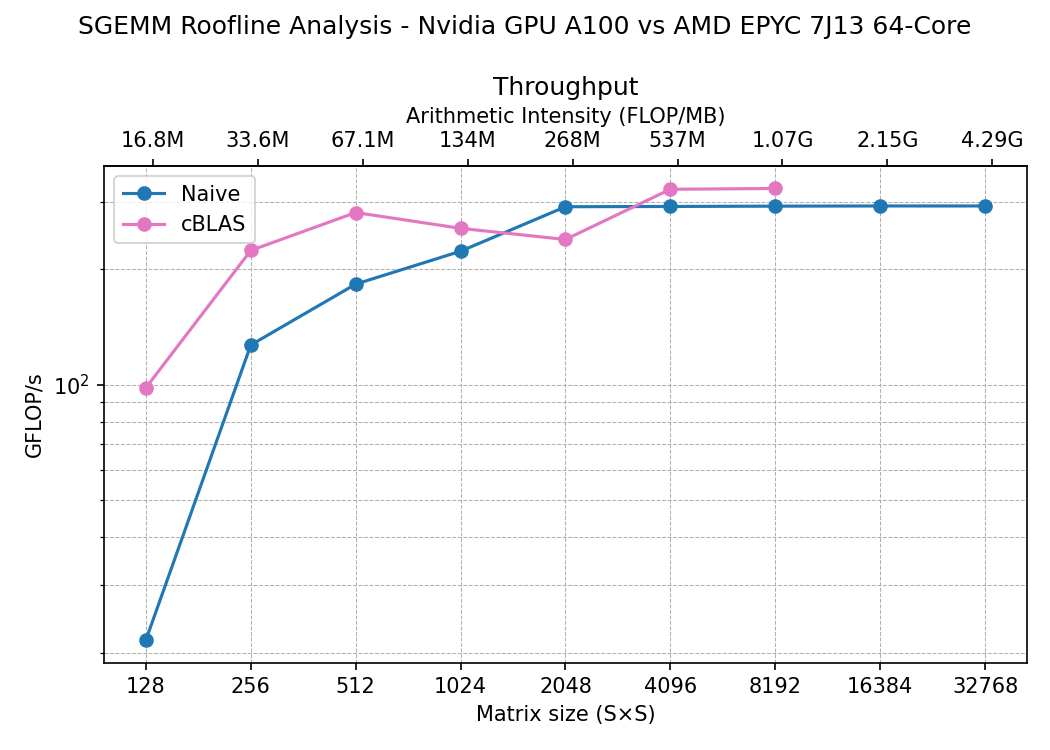
The figure is composed of two graphs, the top one is the roofline calculation, in the bottom x axis we represent the matrix size of A, B and C (square matrices) and in the top x axis the arithmetic intensity. In the y axis we have the compute throughtput or performance for this calculation. In the bottom graph we have the same units for the x axis but in y we represent the gigabytes of data per second transferred.

This result may seem disapointing, the CPU calculation seems to be more performant than the naive GPU kernel. In GPU we barely get to 300 GFLOps/s which is tiny compared to the 19.5 TFLOP/s from the spec sheet.

Memory Coalescing

The next kernel tries to fix the memory access problem by plyaing with the access to the data by warps so that we can coalesce the transfers. We just need to change the variables x and y, the rest remains the same:

template <int BLOCKSIZE>
__global__ void sgemm_coalesced(
    size_t M,
    size_t N,
    size_t K,
    float alpha,
    const float *A,
    const float *B,
    float beta,
    float *C) {

    const uint x = blockIdx.x * BLOCKSIZE + (threadIdx.x / BLOCKSIZE); // 0 .. M-1 (Rows of C)
    const uint y = blockIdx.y * BLOCKSIZE + (threadIdx.x % BLOCKSIZE); // 0 .. N-1 (Columns of C)

    // Warp access e.g. warp 0:
    // x is the same for threads 0..31, y is consecutive for threads 0..31
    // each warp accesses a BLOCKSIZE (32) tile of C, with coalesced accesses to A and C but broadcast acces to B
    // Ref: https://siboehm.com/articles/22/CUDA-MMM

    if (x >= M || y >= N) return;

    float acc = 0.0f;
    for (size_t i = 0; i < K; ++i){
        acc += A[x * K + i] * B[i * N + y];
    }

    C[x * N + y] = alpha * acc + beta * C[x * N + y];
}

called with 1D blocks as:

dim3 gridDim(CEIL_DIV(S, 32), CEIL_DIV(S, 32));
dim3 blockDim(32 * 32);
sgemm_coalesced<32><<<gridDim, blockDim>>>(S, S, S, 1.0f, d_A, d_B, 0.0f, d_C);

Let’s examine the memory accesses for warp 0 as we did in the previous kernel, in this case x and y are:

const uint x = blockIdx.x * BLOCKSIZE + (threadIdx.x / BLOCKSIZE); // 0 .. M-1 (Rows of C)
const uint y = blockIdx.y * BLOCKSIZE + (threadIdx.x % BLOCKSIZE); // 0 .. N-1 (Columns of C)

this means,

x = blockIdx.x*32 + (0..31)/32: Fixed for each warp (0 for warp 0)
y = blockIdx.y*32 + (0..31)%32: Variable within each warp

We access column first in C, which is the order of our memory (row-order).

• A: A[x*K + i]: x fixed, i fixed → same address for every thread on the warp. It’s a broadcast.
• B: B[i*N + y]: i fixed, y varies 0..31 consecutively → addresses i*N+0, i*N+1, ..., i*N+31 — consecutive. Fully coalesced — one 128-byte transaction (4 bytes per float) covers the whole warp.
• C: C[x*N + y]: x fixed, y varies consecutively → same as B, fully coalesced.

So: A broadcast (good), B coalesced (good), C coalesced (good). It’s an improvement from the naive kernel.

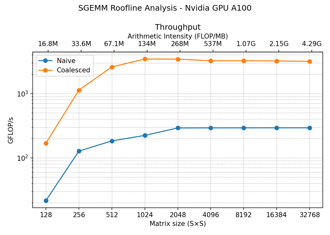
We went from 300 GFLOP/s to 3000 GFLOP/s. That’s a huge improvement!

Tiling

To improve the performance of kenrels a common technique is to use the shared memory, this is a memory that resides closer to the compute. It is a small memory available to all threads in the same block. We can exploit this in our matrix multiplication as rows and columns are accessed several times by many threads. The full kernel is

template <int TILE_SIZE>
__global__ void sgemm_tiled(
    size_t M,             // Number of rows in A and C
    size_t N,             // Number of columns in B and C
    size_t K,             // Number of columns in A and rows in B
    float alpha,       // Scaling factor for the product of A and B
    const float *A,    // [M x K] row-major
    const float *B,    // [K x N] row-major
    float beta,        // Scaling factor for C
    float *C)          // [M x N] row-major  (in-out: C = alpha*A*B + beta*C)
{
    // Declaring the tiles 
    __shared__ float A_tile[TILE_SIZE * TILE_SIZE];
    __shared__ float B_tile[TILE_SIZE * TILE_SIZE];

    // the element of C for this specific thread
    size_t y = blockIdx.y * TILE_SIZE + threadIdx.y;
    size_t x = blockIdx.x * TILE_SIZE + threadIdx.x;

    // we multiply along the K dimension, iterate over this
    size_t n_tiles = (K + TILE_SIZE -1)/TILE_SIZE;

    float acc = .0f;
    for(size_t tile=0; tile<n_tiles; tile++){

        // get tile col from A and tile row for B
        size_t aCol = tile * TILE_SIZE + threadIdx.x;
        size_t bRow = tile * TILE_SIZE + threadIdx.y;

        A_tile[threadIdx.y * TILE_SIZE + threadIdx.x] = (y < M && aCol < K) ? A[y * K + aCol] : 0.0f;
        B_tile[threadIdx.y * TILE_SIZE + threadIdx.x] = (bRow < K && x < N) ? B[bRow * N + x] : 0.0f;

        __syncthreads();

        #pragma unroll
        for (int i = 0; i < TILE_SIZE; ++i)
            acc += A_tile[threadIdx.y * TILE_SIZE + i] * B_tile[i * TILE_SIZE + threadIdx.x];
        __syncthreads();
    }

    if (y < M && x < N)
        C[y * N + x] = alpha * acc + beta * C[y * N + x];
}

and we call this kernel with blocks of 32 by 32 and a 2D grid.

dim3 blockDim(32, 32, 1);
dim3 gridDim(CEIL_DIV(S, blockDim.x), CEIL_DIV(S, blockDim.y));
sgemm_tiled<32><<<gridDim, blockDim>>>(S, S, S, 1.0f, d_A, d_B, 0.0f, d_C);

We declare shared memory tiles of A and B as

__shared__ float A_tile[TILE_SIZE * TILE_SIZE];
__shared__ float B_tile[TILE_SIZE * TILE_SIZE];

those values will be shared accross the block. Now the indexes are similar to the naive kernel. Recall that in our kernel call the TILE_SIZE is the same as the block size.

size_t y = blockIdx.y * TILE_SIZE + threadIdx.y;
size_t x = blockIdx.x * TILE_SIZE + threadIdx.x;

To determine the number of tiles that we need, we divide the common dimension K by the tile sizes. Then we loop on the tiles and let each thread on the tile to load the two elements from the matrices A and B before stopping and waiting for all other threads to finish at __syncthreads() instruction. Once all the elements of the tile are loaded to the shared memory we can perform the multiplication and addition for that tile. After passing through all tiles we finally calculate the new value for that index in C after the loop. Let’s see the performance of this kernel compared to the previous most peformant, the coalesced:

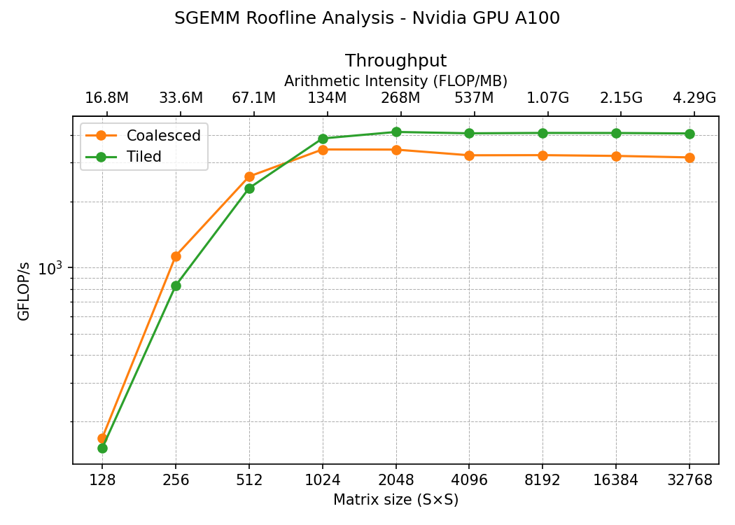
Clearly we have improved the performance, we went from 3000 GFLOPs/s to 4000 GFLOPs/s, not a huge difference but it’s something. Why this kernel is faster?. Well, this time we haven’t used coalesced but we used the shared memory to pull data from the global memory just once, in the naive kernel and the coalesced we were pulling from global many times. Also the loaded elements in the tile are reused many times by the threads in the tile, that makes this operation much faster.

cuBLAS

In this section we use two CUDA libraries for linear algebra, cuBLAS and CUTLASS

cuBLAS is NVIDIA’s closed-source, precompiled BLAS library — you call cublasSgemm() (the equivalent cublas function for our sgemm) and it picks a kernel for you via internal heuristics, drawing on a broad range of pre-tuned kernels to guarantee strong performance across many different problem shapes. It’s a black box: fast and easy to use, but not inspectable or customizable.

The function we need from cuBLAS is cublasSgemm with this signature

cublasStatus_t cublasSgemmEx(cublasHandle_t handle,
    cublasOperation_t transa,
    cublasOperation_t transb,
    int m,
    int n,
    int k,
    const float    *alpha,
    const void     *A,
    cudaDataType_t Atype,
    int lda,
    const void     *B,
    cudaDataType_t Btype,
    int ldb,
    const float    *beta,
    void           *C,
    cudaDataType_t Ctype,
    int ldc)

The call is very similar to the cublas but we need an extra variable called handle. This handle is an opaque object that holds cuBLAS’s library context — basically the state and hardware resources cuBLAS needs to run, allocated on both host and device. The specific call we run is

#include <cublas_v2.h>

cublasHandle_t handle;
cublasCreate(&handle);
cublasSetMathMode(handle, CUBLAS_TF32_TENSOR_OP_MATH);

cublasSgemm(handle,
    CUBLAS_OP_N, CUBLAS_OP_N,
    S, S, S,
    &alpha,
    d_B, S,
    d_A, S,
    &beta,
    d_C, S);

And that’s it, no more secret. Let’s see how the previous tiling kernel compares to cuBLAS

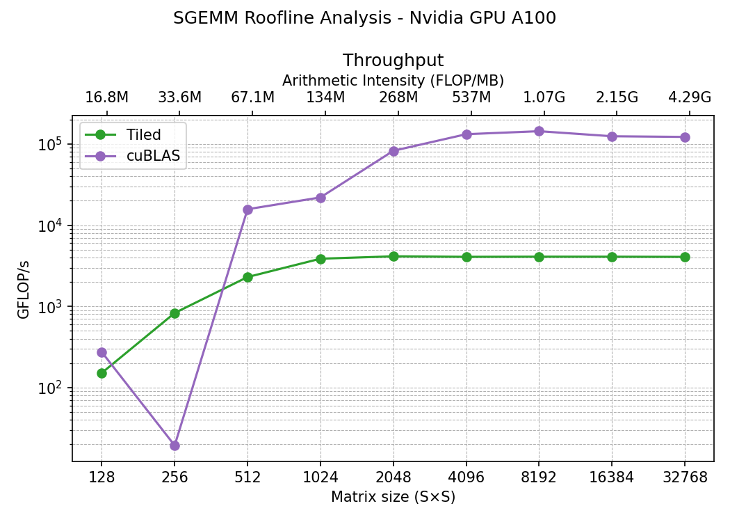
Ok, so we went from 4,000 GFLOP/s to 100,000 GFLOP/s, that’s 25x speedup on the plateau. You may notice here weird stuff happening at 256 matrix size. Launching many calculations on the A100 have the same result for this curve, a drop in performance. As mentioned before, cuBLAS doesn’t contain one single SGEMM implementation — it contains hundreds of them, and it picks among them via internal heuristics tied to problem shape. The other custom implementations used in this post are more consistent in peformance as they are the same algorithm over all ranges of matrix sizes.

CUTLASS

CUTLASS is NVIDIA’s open-source C++ template library for writing GEMM kernels yourself, with reusable building blocks at the device, block, warp, and thread levels. Because you compile only the kernel variants you actually need, binaries stay small — unlike cuBLAS, which ships a large precompiled library covering many cases — but that means you’re responsible for picking and tuning the right kernel for your shape.

The line between cuBLAS and CUTLASS is blurry: cuBLAS internally uses some CUTLASS-derived kernels alongside other sources, mixing kernel origins to keep performance consistent across applications. And on large, well-aligned problems, CUTLASS-built GEMM kernels perform comparably to cuBLAS — the gap mostly shows up at small or oddly-shaped problems, where cuBLAS’s heuristics have more pre-tuned options to fall back on.

In cutlass we will use the GEMM API to code our matrix multiplication. The template cutlass::gemm::device::Gemm requires a set of arguments, some of which are:

using CutlassGemmFP32 = cutlass::gemm::device::Gemm<
    float, cutlass::layout::RowMajor, // A and row major
    float, cutlass::layout::RowMajor, // B and row major
    float, cutlass::layout::RowMajor, // C / D (full float output)
    float,                            // accumulator
    cutlass::arch::OpClassSimt,       // CUDA cores, not tensor cores
    cutlass::arch::Sm80               // Ampere architecture for our A100 GPU
>;

This is the device-level GEMM template class through which CUTLASS GEMM kernels are instantiated. In this configuration we will use OpClassSimt, indicating that we use CUDA cores instead of the much faster tensor cores. Recall that we also specify the architecture, so this library knows how to optimize the operation internally. Next we define the arguments that we need to pass to the cutlass::gemm::device:Gemm class consisting on the sizes and the pointers to the data (and the multipliers alpha and beta).

const float alpha = 1.0f, beta = 0.0f;

CutlassGemmFP32 gemm_op;
CutlassGemmFP32::Arguments args(
    {S, S, S},
    {d_A, S},
    {d_B, S},
    {d_C, S},
    {d_C, S},
    {alpha, beta}
);

Next we create the workspace

// create workspace
size_t workspace_bytes = gemm_op.get_workspace_size(args);
void* workspace = nullptr;
if (workspace_bytes)
    cudaMalloc(&workspace, workspace_bytes);

and we launch the calculation

// launch operation
cutlass::Status s = gemm_op(args, workspace);
if (s != cutlass::Status::kSuccess) {
    fprintf(stderr, "CUTLASS error %d\n", (int)s);
    exit(EXIT_FAILURE);
}
cudaDeviceSynchronize();

In terms of benchmarking we can compare with cuBLAs:

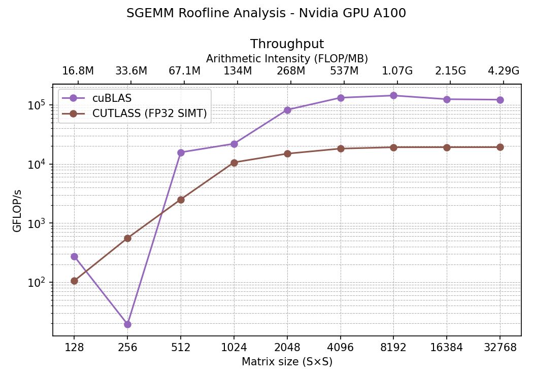
Surprisingly (or not…), cuBLAS achieves larger performance. This is because we specifically told CUTLASS to use CUDA processors instead of CUDA cores, cuBLAS being a much higher level library is probably using tensor cores directly. These tensor cores are much faster than regular GPU cores and they are perfect for matrix multiplication. Their drawback is that they compute half precision floating points (FP16) and this means we get lower precision. However there are ways to compute FP32 in tensor cores still. In the repository you will find that we also use cutlass::arch::OpClassTensorOp to force CUTLASS to use the tensor cores and in one case we cast A and B to half precision (FP16) and in the other we need to reinterpret the floats to cutlass::tfloat32_t (TF32) type. Skipping details here are the comparison between these implementations:

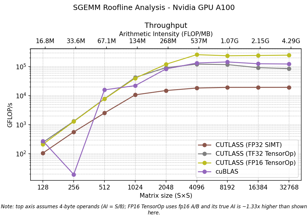
Note that with TF32 we reach the same performance as in cuBLAS at plateau, about $10^5$. That seems to indicate that in our case cuBLAS decides to use tensor cores and TF32 casting. However tensor cores are designed for FP16, it’s natural that we achieve the higher performance in this case. Recall that since we cap the precision to half, also the arithmetic intensity has to be scaled, something that is not shown in the graph, the true arithmetic intensity for FP16 is 1.33 times larger than the shown in the x axis. In any case at saturation (plateau) the FP16 wins on throughput.

Comparison all kernels

Finally we can compare all the kernels calculated. In the following graph we show on top the roofline calculated curves we have been showing but all in the same place and in the bottom the memory transfer (memory bandwidth) as a function of the time.

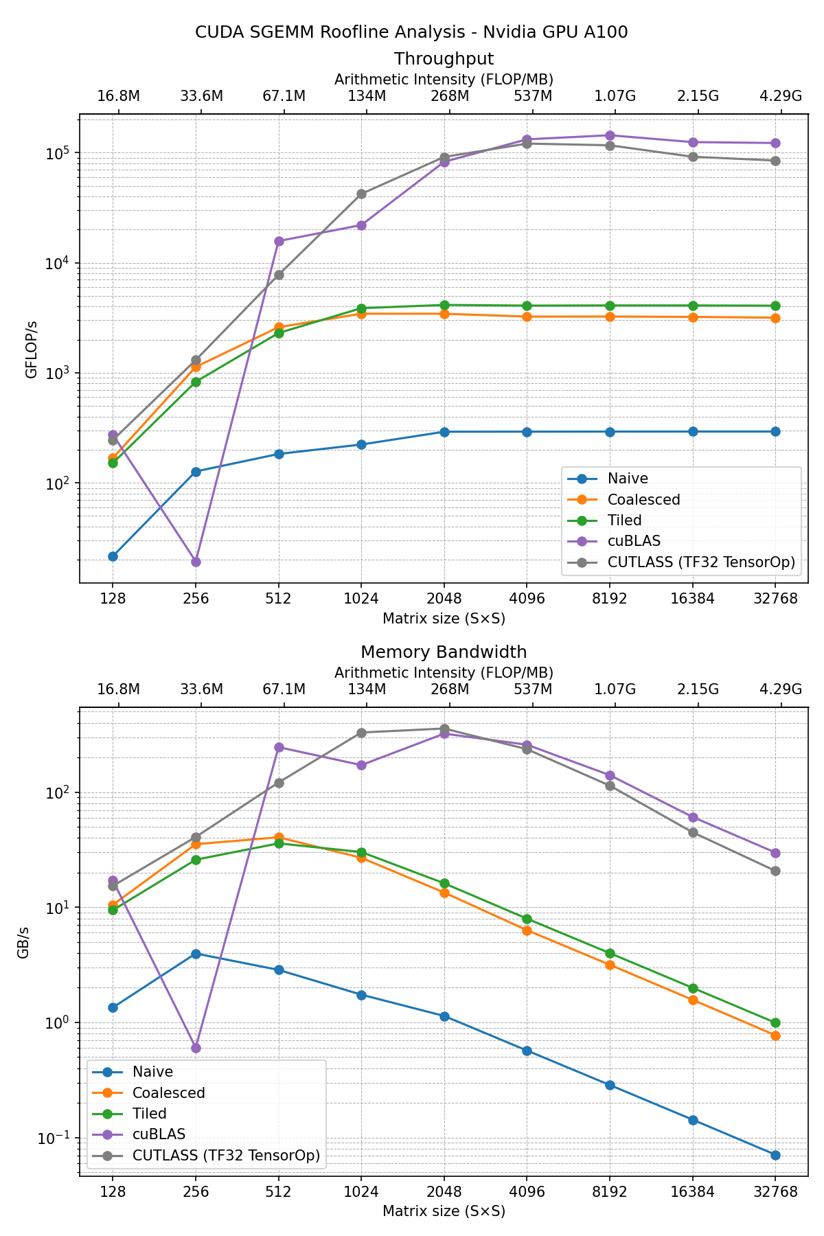
The golden standard is the cuBLAS implementation, but according to the previous section that is very close or equivalent to the CUTLASS TF32 implementation (using tensor cores and single floating point precision). These are extremely useful libraries that many experts have been years developing. We can’t get much better than this with pure kernel programming.